User libraries is a sub-package where useful Python modules contributed by users are stored.
Optimisation - Taguchi’s method
Information
Author/Contact: Craig Warren (craig.warren@northumbria.ac.uk), Northumbria University, UK
License: Creative Commons Attribution-ShareAlike 4.0 International License
Attribution/cite: Warren, C., Giannopoulos, A. (2011). Creating finite-difference time-domain models of commercial ground-penetrating radar antennas using Taguchi’s optimization method. Geophysics, 76(2), G37-G47. (http://dx.doi.org/10.1190/1.3548506)
The package features an optimisation technique based on Taguchi’s method. It allows users to define parameters in an input file and optimise their values based on a fitness function, for example it can be used to optimise material properties or geometry in a simulation.
Warning
This package combines a number of advanced features and should not be used without knowledge and familiarity of the underlying techniques. It requires:
- Knowledge of Python to contruct an input file to use with the optimisation
- Familiarity of optimisation techniques, and in particular Taguchi’s method
- Careful sanity checks to be made throughout the process
Taguchi’s method
Taguchi’s method is based on the concept of the Orthogonal Array (OA) and has the following advantages:
- Simple to implement
- Effective in reduction of experiments
- Fast convergence speed
- Global optimum results
- Independence from initial values of optimisation parameters
Details of Taguchi’s method in the context of electromagnetics can be found in [WEN2007a] and [WEN2007b].
Package overview
antenna_bowtie_opt.in
fitness_functions.py
OA_9_4_3_2.npy
OA_18_7_3_2.npy
plot_results.py
antenna_bowtie_opt.inis a example model of a bowtie antenna where values of loading resistors are optimised.fitness_functions.pyis a module containing fitness functions. There are some pre-built ones but users should add their own here.OA_9_4_3_2.npyandOA_18_7_3_2.npyare NumPy archives containing pre-built OAsplot_results.pyis a module for plotting the results, such as parameter values and convergence history, from an optimisation process when it has completed.
Implementation
The process by which Taguchi’s method optimises parameters is illustrated in the following figure:
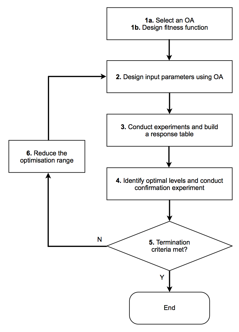
Fig. 29 Process associated with Taguchi’s method.
In stage 1a, one of the 2 pre-built OAs will automatically be chosen depending on the number of parameters to optimise. Currently, up to 7 independent parameters can be optimised, although a method to construct OAs of any size is under testing.
In stage 1b, a fitness function is required to set a goal against which to compare results from the optimisation process. A number of pre-built fitness functions can be found in the fitness_functions.py module, e.g. minvalue, maxvalue and xcorr. Users can also easily add their own fitness functions to this module. All fitness functions must take two arguments:
filenamea string containing the full path and filename of the output fileargsa dictionary which can contain any number of additional arguments for the function, e.g. names of outputs (rxs) in the model
Additionally, all fitness functions must return a single fitness value which the optimsation process will aim to maximise.
Stages 2-6 are iterated through by the optimisation process.
Parameters and settings for the optimisation process are specified within a special Python block defined by #taguchi and #end_taguchi in the input file. The parameters to optimise must be defined in a dictionary named optparams and their initial ranges specified as lists with lower and upper values. The fitness function, it’s parameters, and a stopping value are defined in dictionary named fitness which has keys for:
namea string that is the name of the fitness function to be usedargsa dictionary containing arguments to be passed to the fitness function. Withinargsthere must be a key calledoutputswhich contains a string or list of the names of one or more outputs (rxs) in the modelstopa value from the fitness function which when exceeded the optimisation should stop
Optionally a variable called maxiterations maybe specified which will set a maximum number of iterations after which the optimisation process will terminate irrespective of any other criteria. If it is not specified it defaults to a maximum of 20 iterations.
There is also a builtin criterion to terminate the optimisation process is successive fitness values are within 0.1% of one another.
How to use the package
The package requires #python and #end_python to be used in the input file, as well as #taguchi and #end_taguchi for specifying parameters and setting for the optimisation process. A Taguchi optimisation is run using the command line option --opt-taguchi.
Example
The following example demonstrates using the Taguchi optimisation process to optimise values of loading resistors used in a bowtie antenna. The example is slighty contrived as the goal is simply to find values for the resistors that produces a maximum absolute amplitude in the response from the antenna. We already know this should occur when the values of the resistors are at a minimum. Nevertheless, it is useful to illustrate the optimisation process and how to use it.
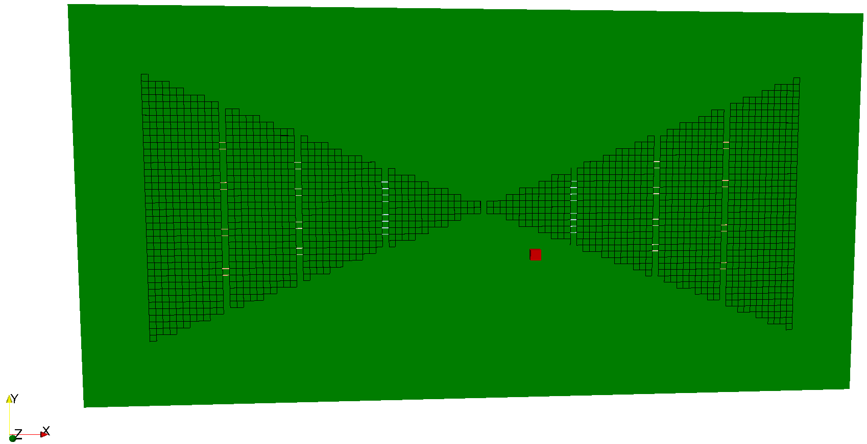
Fig. 30 FDTD geometry mesh showing bowtie antenna with slots and loading resistors.
The bowtie design features three vertical slots (y-direction) in each arm of the bowtie. Each slot has different loading resistors, but within each slot there are four resistors of the same value. A resistor is modelled as two parallel edges of a cell. The bowtie is placed on a lossless substrate of relative permittivity 4.8. The antenna is modelled in free space, and an output point of the electric field (named Ex60mm) is specified at a distance of 60mm from the feed of the bowtie (red coloured cell).
1 2 3 4 5 6 7 8 9 10 11 12 13 14 15 16 17 18 19 20 21 22 23 24 25 26 27 28 29 30 31 32 33 34 35 36 37 38 39 40 41 42 43 44 45 46 47 48 49 50 51 52 53 54 55 56 57 58 59 60 61 62 63 64 65 66 67 68 69 70 71 72 73 74 75 76 77 78 79 80 81 82 83 84 85 86 87 88 89 90 91 92 | #taguchi:
optparams['resinner'] = [0.1, 1000]
optparams['resmiddle'] = [0.1, 1000]
optparams['resouter'] = [0.1, 1000]
fitness = {'name': 'min_max_value', 'stop': 10, 'args': {'type': 'absmax', 'outputs': 'Ex60mm'}}
#end_taguchi:
#python:
import numpy as np
from gprMax.input_cmd_funcs import *
title = 'antenna_bowtie_opt'
print('#title: {}'.format(title))
domain = domain(0.180, 0.120, 0.160)
dxdydz = dx_dy_dz(0.001, 0.001, 0.001)
timewindow = time_window(5e-9)
fr4_dims = (0.120, 0.060, 0.002)
bowtie_dims = (0.050, 0.040) # Length, height
flare_angle = np.arctan((bowtie_dims[1]/2) / bowtie_dims[0])
tx_pos = (domain[0]/2, domain[1]/2, 0.050)
# Vertical slot positions, relative to feed position, i.e. txpos[0]
vcut_pos = (0.014, 0.027, 0.038)
# Loading resistor values
res = np.array([optparams['resinner'], optparams['resmiddle'], optparams['resouter']])
rescond = ((1 / res) * (dxdydz[1] / (dxdydz[0] * dxdydz[2]))) / 2 # Divide by number of parallel edges per resistor
# Materials
material(4.8, 0, 1, 0, 'fr4')
for i in range(len(res)):
material(1, rescond[i], 1, 0, 'res' + str(i + 1))
# Source excitation and type
print('#waveform: gaussian 1 2e9 mypulse')
print('#transmission_line: x {:g} {:g} {:g} 50 mypulse'.format(tx_pos[0], tx_pos[1], tx_pos[2]))
# Output point - distance from tx_pos in z direction
print('#rx: {:g} {:g} {:g} Ex60mm Ex'.format(tx_pos[0], tx_pos[1], tx_pos[2] + 0.060))
# Bowtie - upper x half
triangle(tx_pos[0], tx_pos[1], tx_pos[2], tx_pos[0] + bowtie_dims[0], tx_pos[1] - bowtie_dims[1]/2, tx_pos[2], tx_pos[0] + bowtie_dims[0], tx_pos[1] + bowtie_dims[1]/2, tx_pos[2], 0, 'pec')
# Bowtie - upper x half - vertical cuts
for i in range(len(vcut_pos)):
for j in range(int(bowtie_dims[1] / dxdydz[2])):
edge(tx_pos[0] + vcut_pos[i], tx_pos[1] - bowtie_dims[1]/2 + j * dxdydz[1], tx_pos[2], tx_pos[0] + vcut_pos[i] + dxdydz[0], tx_pos[1] - bowtie_dims[1]/2 + j * dxdydz[1], tx_pos[2], 'free_space')
# Bowtie - upper x half - vertical cuts - loading
for i in range(len(vcut_pos)):
gap = ((vcut_pos[i] * np.tan(flare_angle) * 2) - 4*dxdydz[1]) / 5
edge(tx_pos[0] + vcut_pos[i], tx_pos[1] - (1.5 * gap) - dxdydz[1], tx_pos[2], tx_pos[0] + vcut_pos[i] + dxdydz[0], tx_pos[1] - (1.5 * gap) - dxdydz[1], tx_pos[2], 'res' + str(i + 1))
edge(tx_pos[0] + vcut_pos[i], tx_pos[1] - (1.5 * gap) - 2*dxdydz[1], tx_pos[2], tx_pos[0] + vcut_pos[i] + dxdydz[0], tx_pos[1] - (1.5 * gap) - 2*dxdydz[1], tx_pos[2], 'res' + str(i + 1))
edge(tx_pos[0] + vcut_pos[i], tx_pos[1] - (0.5 * gap), tx_pos[2], tx_pos[0] + vcut_pos[i] + dxdydz[0], tx_pos[1] - (0.5 * gap), tx_pos[2], 'res' + str(i + 1))
edge(tx_pos[0] + vcut_pos[i], tx_pos[1] - (0.5 * gap) - dxdydz[1], tx_pos[2], tx_pos[0] + vcut_pos[i] + dxdydz[0], tx_pos[1] - (0.5 * gap) - dxdydz[1], tx_pos[2], 'res' + str(i + 1))
edge(tx_pos[0] + vcut_pos[i], tx_pos[1] + (0.5 * gap), tx_pos[2], tx_pos[0] + vcut_pos[i] + dxdydz[0], tx_pos[1] + (0.5 * gap), tx_pos[2], 'res' + str(i + 1))
edge(tx_pos[0] + vcut_pos[i], tx_pos[1] + (0.5 * gap) + dxdydz[1], tx_pos[2], tx_pos[0] + vcut_pos[i] + dxdydz[0], tx_pos[1] + (0.5 * gap) + dxdydz[1], tx_pos[2], 'res' + str(i + 1))
edge(tx_pos[0] + vcut_pos[i], tx_pos[1] + (1.5 * gap) + dxdydz[1], tx_pos[2], tx_pos[0] + vcut_pos[i] + dxdydz[0], tx_pos[1] + (1.5 * gap) + dxdydz[1], tx_pos[2], 'res' + str(i + 1))
edge(tx_pos[0] + vcut_pos[i], tx_pos[1] + (1.5 * gap) + 2*dxdydz[1], tx_pos[2], tx_pos[0] + vcut_pos[i] + dxdydz[0], tx_pos[1] + (1.5 * gap) + 2*dxdydz[1], tx_pos[2], 'res' + str(i + 1))
# Bowtie - lower x half
triangle(tx_pos[0] + dxdydz[0], tx_pos[1], tx_pos[2], tx_pos[0] - bowtie_dims[0], tx_pos[1] - bowtie_dims[1]/2, tx_pos[2], tx_pos[0] - bowtie_dims[0], tx_pos[1] + bowtie_dims[1]/2, tx_pos[2], 0, 'pec')
# Bowtie - lower x half - cuts for loading
for i in range(len(vcut_pos)):
for j in range(int(bowtie_dims[1] / dxdydz[2])):
edge(tx_pos[0] - vcut_pos[i] - dxdydz[0], tx_pos[1] - bowtie_dims[1]/2 + j * dxdydz[1], tx_pos[2], tx_pos[0] - vcut_pos[i], tx_pos[1] - bowtie_dims[1]/2 + j * dxdydz[1], tx_pos[2], 'free_space')
# Bowtie - lower x half - vertical cuts - loading
for i in range(len(vcut_pos)):
gap = ((vcut_pos[i] * np.tan(flare_angle) * 2) - 4*dxdydz[1]) / 5
edge(tx_pos[0] - vcut_pos[i] - dxdydz[0], tx_pos[1] - (1.5 * gap) - dxdydz[1], tx_pos[2], tx_pos[0] - vcut_pos[i], tx_pos[1] - (1.5 * gap) - dxdydz[1], tx_pos[2], 'res' + str(i + 1))
edge(tx_pos[0] - vcut_pos[i] - dxdydz[0], tx_pos[1] - (1.5 * gap) - 2*dxdydz[1], tx_pos[2], tx_pos[0] - vcut_pos[i], tx_pos[1] - (1.5 * gap) - 2*dxdydz[1], tx_pos[2], 'res' + str(i + 1))
edge(tx_pos[0] - vcut_pos[i] - dxdydz[0], tx_pos[1] - (0.5 * gap), tx_pos[2], tx_pos[0] - vcut_pos[i], tx_pos[1] - (0.5 * gap), tx_pos[2], 'res' + str(i + 1))
edge(tx_pos[0] - vcut_pos[i] - dxdydz[0], tx_pos[1] - (0.5 * gap) - dxdydz[1], tx_pos[2], tx_pos[0] - vcut_pos[i], tx_pos[1] - (0.5 * gap) - dxdydz[1], tx_pos[2], 'res' + str(i + 1))
edge(tx_pos[0] - vcut_pos[i] - dxdydz[0], tx_pos[1] + (0.5 * gap), tx_pos[2], tx_pos[0] - vcut_pos[i], tx_pos[1] + (0.5 * gap), tx_pos[2], 'res' + str(i + 1))
edge(tx_pos[0] - vcut_pos[i] - dxdydz[0], tx_pos[1] + (0.5 * gap) + dxdydz[1], tx_pos[2], tx_pos[0] - vcut_pos[i], tx_pos[1] + (0.5 * gap) + dxdydz[1], tx_pos[2], 'res' + str(i + 1))
edge(tx_pos[0] - vcut_pos[i] - dxdydz[0], tx_pos[1] + (1.5 * gap) + dxdydz[1], tx_pos[2], tx_pos[0] - vcut_pos[i], tx_pos[1] + (1.5 * gap) + dxdydz[1], tx_pos[2], 'res' + str(i + 1))
edge(tx_pos[0] - vcut_pos[i] - dxdydz[0], tx_pos[1] + (1.5 * gap) + 2*dxdydz[1], tx_pos[2], tx_pos[0] - vcut_pos[i], tx_pos[1] + (1.5 * gap) + 2*dxdydz[1], tx_pos[2], 'res' + str(i + 1))
# PCB
box(tx_pos[0] - fr4_dims[0]/2, tx_pos[1] - fr4_dims[1]/2, tx_pos[2] - fr4_dims[2], tx_pos[0] + fr4_dims[0]/2, tx_pos[1] + fr4_dims[1]/2, tx_pos[2], 'fr4')
# Detailed geometry view of PCB and bowtie
#geometry_view(tx_pos[0] - fr4_dims[0]/2, tx_pos[1] - fr4_dims[1]/2, tx_pos[2] - fr4_dims[2], tx_pos[0] + fr4_dims[0]/2, tx_pos[1] + fr4_dims[1]/2, tx_pos[2] + dxdydz[2], dxdydz[0], dxdydz[1], dxdydz[2], title + '_tx', type='f')
# Geometry view of entire domain
#geometry_view(0, 0, 0, domain[0], domain[1], domain[2], dxdydz[0], dxdydz[1], dxdydz[2], title)
#end_python:
|
The first part of the input file (lines 1-6) contains the parameters to optimise, their initial ranges, and fitness function information for the optimisation process. Three parameters representing the resistor values are defined with ranges between 0.1 \(\Omega\) and 1 \(k\Omega\). A pre-built fitness function called min_max_value is specified with a stopping criterion of 10V/m. Arguments for the min_max_value function are type given as absmax, i.e. the maximum absolute values, and the output point in the model that will be used in the optimisation is specified as having the name Ex60mm.
The next part of the input file (lines 8-92) contains the model. For the most part there is nothing special about the way the model is defined - a mixture of Python, NumPy and functional forms of the input commands (available by importing the module input_cmd_funcs) are used. However, it is worth pointing out how the values of the parameters to optimise are accessed. On line 29 a NumPy array of the values of the resistors is created. The values are accessed using their names as keys to the optparams dictionary. On line 30 the values of the resistors are converted to conductivities, which are used to create new materials (line 34-35). The resistors are then built by applying the materials to cell edges (e.g. lines 55-62). The output point in the model in specifed with the name Ex60mm and as having only an Ex field output (line 42).
The optimisation process is run on the model using the --opt-taguchi command line flag.
python -m gprMax user_libs/optimisation_taguchi/antenna_bowtie_opt.in --opt-taguchi
Results
When the optimisation has completed a summary will be printed showing histories of the parameter values and the fitness metric. These values are also saved (pickled) to file and can be plotted using the plot_results.py module, for example:
python -m user_libs.optimisation_taguchi.plot_results user_libs/optimisation_taguchi/antenna_bowtie_opt_hist.pickle
Optimisations summary for: antenna_bowtie_opt_hist.pickle
Number of iterations: 4
History of fitness values: [4.2720928, 5.68856, 5.7023263, 5.7023263]
History of parameter values:
resinner [250.07498, 0.87031555, 0.1, 0.1]
resmiddle [250.07498, 0.87031555, 0.1, 0.1]
resouter [250.07498, 0.87031555, 0.1, 0.1]
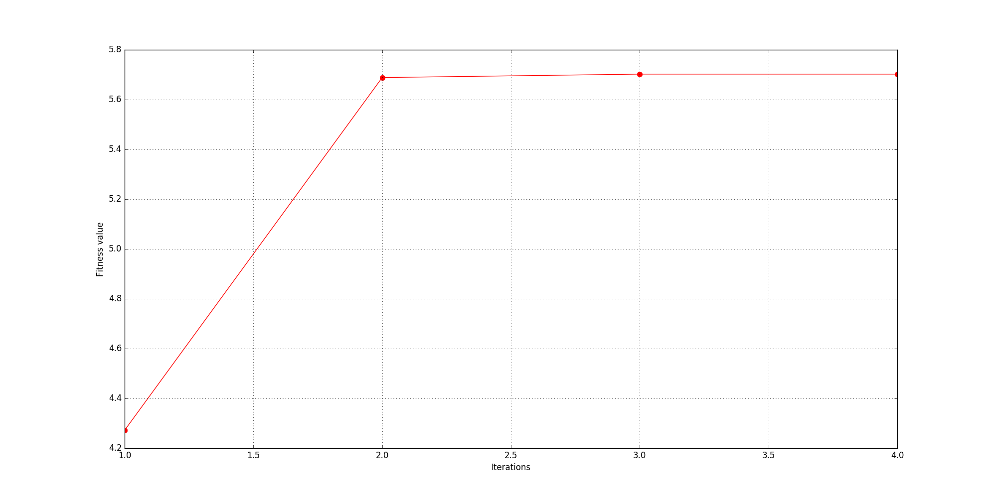
Fig. 31 History of values of fitness metric (absolute maximum).
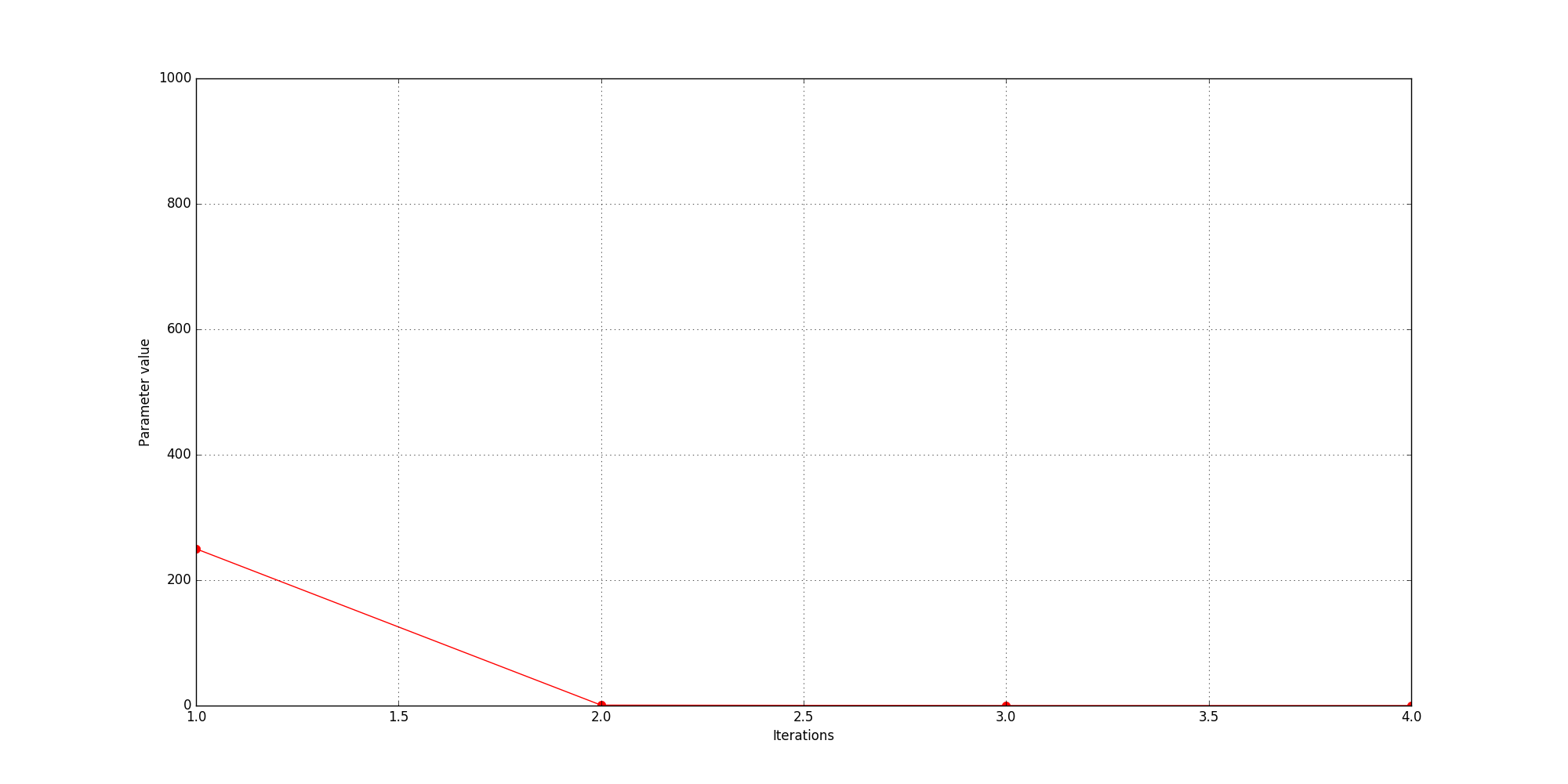
Fig. 32 History of values of parameters - resinner, resmiddle, and resouter (in this case they are all identical).
The optimisation process terminated after 4 iterations because succcessive fitness values were within 0.1% of one another. A maximum absolute amplitude value of 5.7 V/m was achieved when the three resistors had values of 0.1 \(\Omega\).